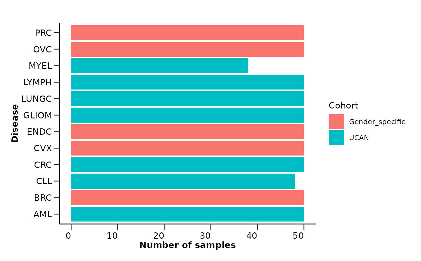
hd_qc_summary() summarizes the quality control results of the input data and metadata.
It returns general information about the datasets, missing value information,
protein-protein correlations, and metadata summary visualizations.
Usage
hd_qc_summary(
  dat,
  metadata = NULL,
  variable,
  palette = NULL,
  unique_threshold = 5,
  cor_threshold = 0.8,
  cor_method = "pearson",
  max_heatmap_features = 1000,
  verbose = TRUE
)
Arguments
- dat
An HDAnalyzeR object or a dataset in wide format and sample ID as its first column.
- metadata
A dataset containing the metadata information with the sample ID as the first column. If a HDAnalyzeR object is provided, this parameter is not needed.
- variable
The name of the metadata variable (column) containing the different classes (for example the column that contains your case and control groups).
- palette
A list of color palettes for the plots. The names of the list should match the column names in the metadata. Default is NULL.
- unique_threshold
The threshold to consider a numeric variable as categorical. Default is 5.
- cor_threshold
The threshold to consider a protein-protein correlation as high. Default is 0.8.
- cor_method
The method to calculate the correlation. Default is "pearson". Other options are "spearman" and "kendall".
- max_heatmap_features
The largest number of features to draw a correlation heatmap for. Default is 1000. Above this the correlation matrix and the reported pairs are still returned, but the heatmap is skipped, since clustering that many features is prohibitively slow and the plot is unreadable.
- verbose
Whether to print the summary. Default is TRUE.
Examples
# Create the HDAnalyzeR object providing the data and metadata
hd_object <- hd_initialize(example_data,
example_metadata |> dplyr::select(-Sample))
# Run the quality control summary
qc_res <- hd_qc_summary(hd_object,
variable = "Disease",
palette = list(Disease = "cancers12", Sex = "sex"),
cor_threshold = 0.7,
verbose = TRUE)
#> Summary:
#> Note: In case of long output, only the first 10 rows are shown. To see the rest display the object with view()
#> Number of samples: 586
#> Number of variables: 101
#> --------------------------------------
#> categorical: 1
#> continuous: 100
#> --------------------------------------
#> NA percentage in each column:
#> # A tibble: 10 × 2
#> column na_percentage
#> <chr> <dbl>
#> 1 ACE2 6.1
#> 2 ACTA2 6.1
#> 3 ACTN4 6.1
#> 4 ADAM15 6.1
#> 5 ADAMTS16 6.1
#> 6 ADH4 6.1
#> 7 AKR1C4 6.1
#> 8 AMBN 6.1
#> 9 AMN 6.1
#> 10 AOC1 6.1
#> ... and 81 more rows.
#> --------------------------------------
#> NA percentage in each row:
#> # A tibble: 10 × 2
#> DAid na_percentage
#> <chr> <dbl>
#> 1 DA00450 57.4
#> 2 DA00482 53.5
#> 3 DA00542 53.5
#> 4 DA00003 50.5
#> 5 DA00463 46.5
#> 6 DA00116 43.6
#> 7 DA00475 42.6
#> 8 DA00578 42.6
#> 9 DA00443 41.6
#> 10 DA00476 35.6
#> ... and 134 more rows.
#> --------------------------------------
#> Protein-protein correlations above 0.7:
#> # A tibble: 6 × 3
#> Protein1 Protein2 Correlation
#> <chr> <chr> <dbl>
#> 1 ATP5IF1 AIFM1 0.76
#> 2 AXIN1 ARHGEF12 0.76
#> 3 AIFM1 ATP5IF1 0.76
#> 4 ARHGEF12 AXIN1 0.76
#> 5 ARHGEF12 AIFM1 0.71
#> 6 AIFM1 ARHGEF12 0.71
#> --------------------------------------
#> Summary:
#> Note: In case of long output, only the first 10 rows are shown. To see the rest display the object with view()
#> Number of samples: 586
#> Number of variables: 8
#> --------------------------------------
#> categorical: 6
#> continuous: 2
#> --------------------------------------
#> NA percentage in each column:
#> # A tibble: 1 × 2
#> column na_percentage
#> <chr> <dbl>
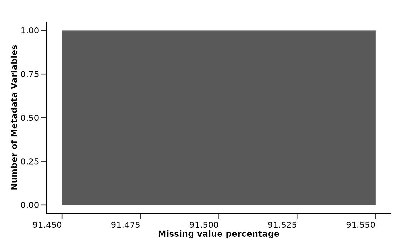
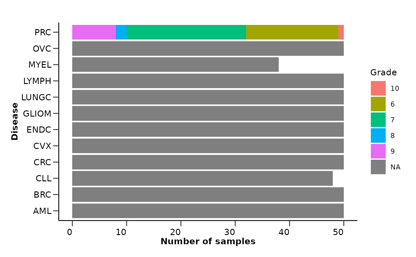
#> 1 Grade 91.5
#> --------------------------------------
#> NA percentage in each row:
#> # A tibble: 10 × 2
#> DAid na_percentage
#> <chr> <dbl>
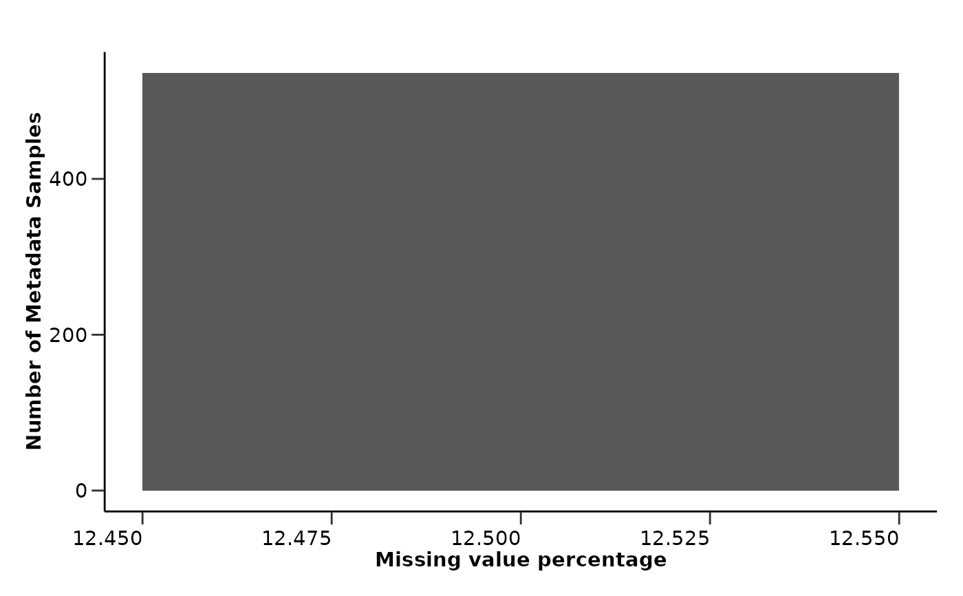
#> 1 DA00001 12.5
#> 2 DA00002 12.5
#> 3 DA00003 12.5
#> 4 DA00004 12.5
#> 5 DA00005 12.5
#> 6 DA00006 12.5
#> 7 DA00007 12.5
#> 8 DA00008 12.5
#> 9 DA00009 12.5
#> 10 DA00010 12.5
#> ... and 526 more rows.
#> --------------------------------------
# Data summary -------------------------------------------------------------
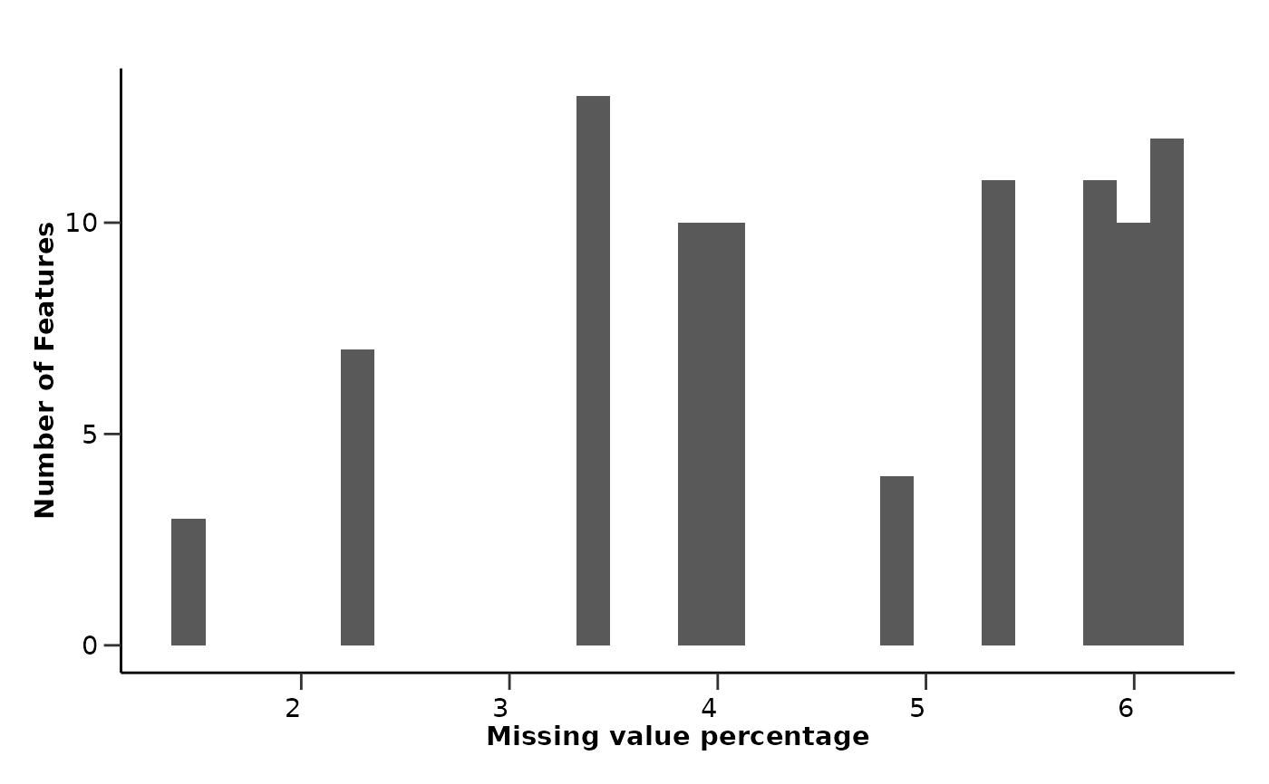
qc_res$data_summary$na_col_hist
#> `stat_bin()` using `bins = 30`. Pick better value `binwidth`.
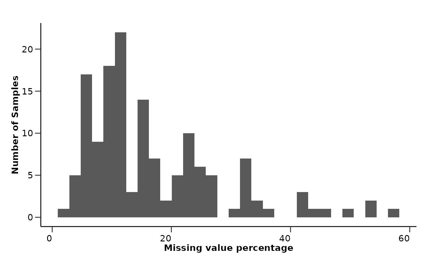
 qc_res$data_summary$na_row_hist
#> `stat_bin()` using `bins = 30`. Pick better value `binwidth`.
qc_res$data_summary$na_row_hist
#> `stat_bin()` using `bins = 30`. Pick better value `binwidth`.
 qc_res$data_summary$cor_results
#> # A tibble: 6 × 3
#> Protein1 Protein2 Correlation
#> <chr> <chr> <dbl>
#> 1 ATP5IF1 AIFM1 0.76
#> 2 AXIN1 ARHGEF12 0.76
#> 3 AIFM1 ATP5IF1 0.76
#> 4 ARHGEF12 AXIN1 0.76
#> 5 ARHGEF12 AIFM1 0.71
#> 6 AIFM1 ARHGEF12 0.71
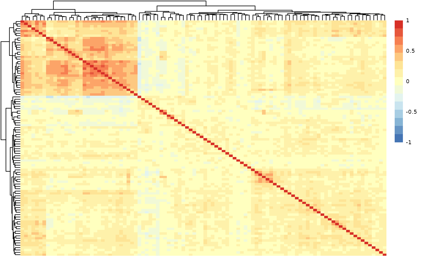
qc_res$data_summary$cor_heatmap
qc_res$data_summary$cor_results
#> # A tibble: 6 × 3
#> Protein1 Protein2 Correlation
#> <chr> <chr> <dbl>
#> 1 ATP5IF1 AIFM1 0.76
#> 2 AXIN1 ARHGEF12 0.76
#> 3 AIFM1 ATP5IF1 0.76
#> 4 ARHGEF12 AXIN1 0.76
#> 5 ARHGEF12 AIFM1 0.71
#> 6 AIFM1 ARHGEF12 0.71
qc_res$data_summary$cor_heatmap
 # Metadata summary ---------------------------------------------------------
qc_res$metadata_summary$na_col_hist
#> `stat_bin()` using `bins = 30`. Pick better value `binwidth`.
# Metadata summary ---------------------------------------------------------
qc_res$metadata_summary$na_col_hist
#> `stat_bin()` using `bins = 30`. Pick better value `binwidth`.
 qc_res$metadata_summary$na_row_hist
#> `stat_bin()` using `bins = 30`. Pick better value `binwidth`.
qc_res$metadata_summary$na_row_hist
#> `stat_bin()` using `bins = 30`. Pick better value `binwidth`.
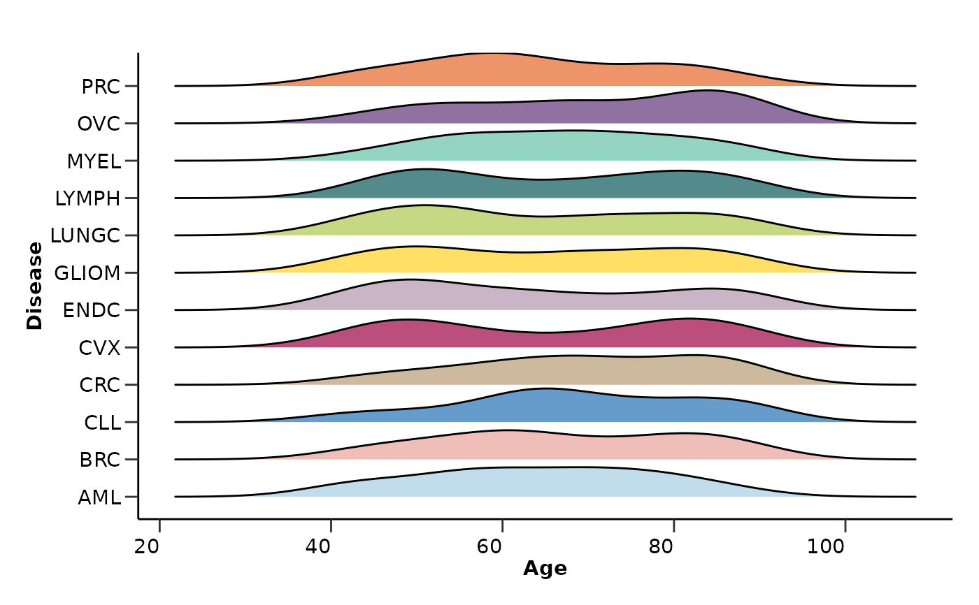
 qc_res$metadata_summary$Age
#> Picking joint bandwidth of 6.06
qc_res$metadata_summary$Age
#> Picking joint bandwidth of 6.06
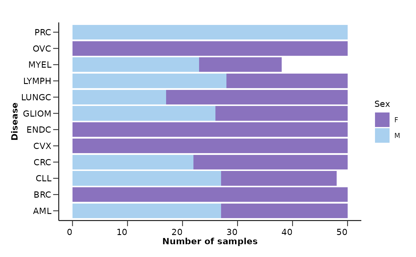
 qc_res$metadata_summary$Sex
 qc_res$metadata_summary$BMI
#> Picking joint bandwidth of 1.77
qc_res$metadata_summary$BMI
#> Picking joint bandwidth of 1.77
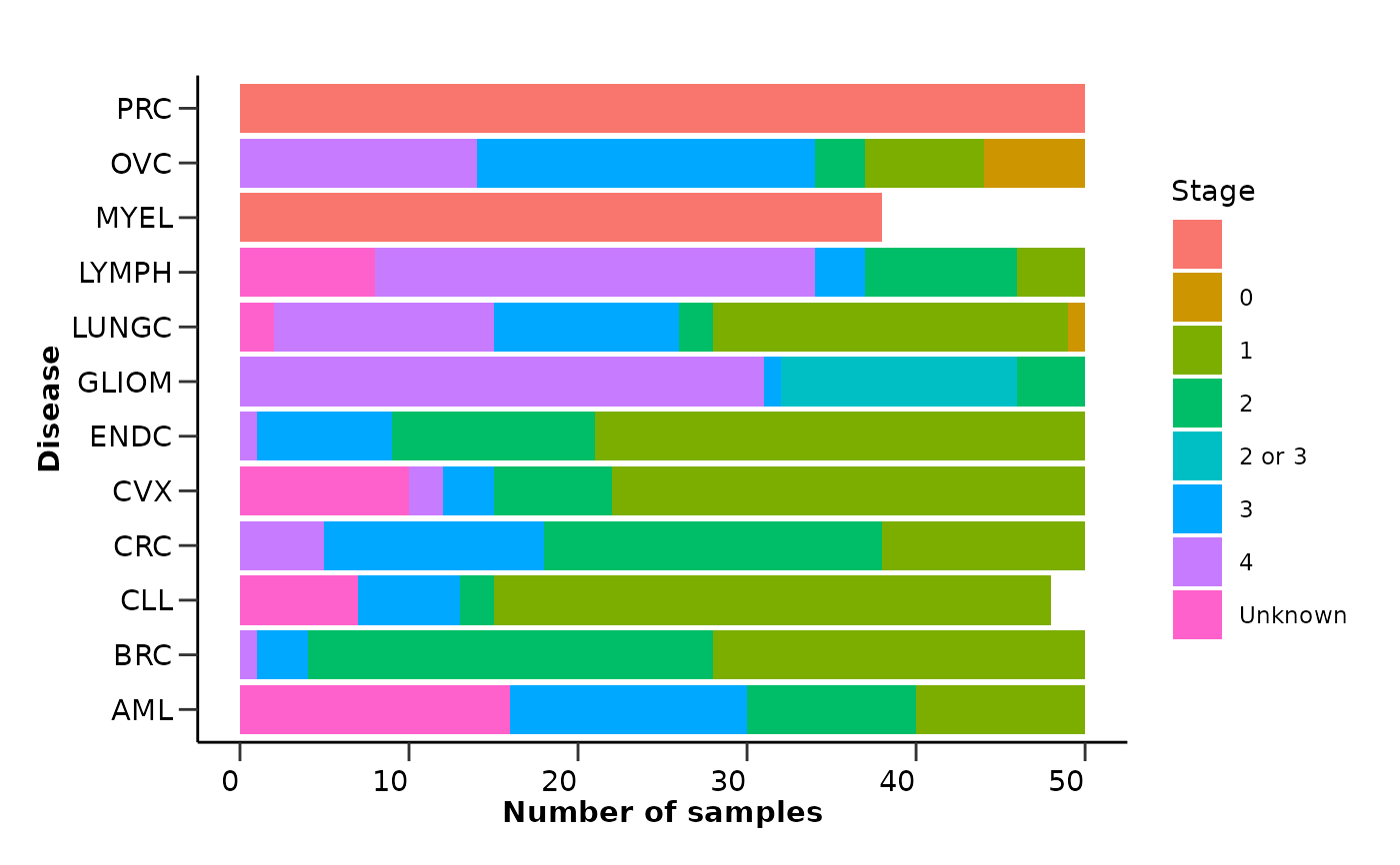
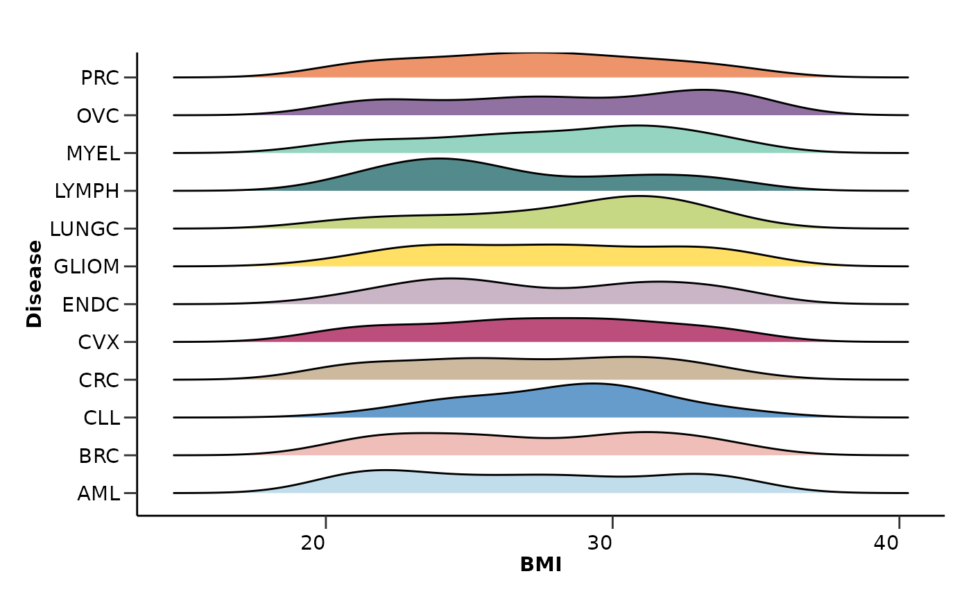 qc_res$metadata_summary$Stage
 qc_res$metadata_summary$Grade
 qc_res$metadata_summary$Cohort